LAUREL: Location-Attuned Uncertainty-Robust Electric-vehicle Load-simulator

This repository implements the LAUREL model described in:

Passow, F. H., & Rajagopal, R. (2026). Prioritizing uncertainty-robust indicators to inform proactive substation upgrades for charging electric heavy-duty trucks. Applied Energy (submitted March 2026).

The specific use of the LAUREL model demonstrated here estimates e-HDT charging load profiles for each of the ~52,000 electrical substations in the continental U.S. across 1024 plausible future states of the world (SoWs) representing 2035 conditions. It identifies which substations grid operators should consider proactively upgrading for e-HDT charging, and what techno-economic indicators signal when such an upgrade may become necessary — findings that are assessed for robustness to uncertainty across all 1024 SoWs.

Background 

Electric heavy-duty trucks (e-HDTs) will require geographically concentrated, high-power charging that will stress electric distribution infrastructure — particularly substations, which can take years and millions of dollars to upgrade. This model was built to answer: which substations should grid operators proactively upgrade, and what observable conditions should trigger that decision?

Our approach uses a continent-scale telematics dataset of ~69,000 diesel HDTs (International, Inc., April–November 2023) as the behavioral foundation. We simulate electrified versions of these vehicles across 1024 quasi-random combinations of key uncertain parameters (adoption rates, energy consumption, charger power, battery reserve). For each combination, we assemble 30-minute load profiles for every substation in the continental U.S. Findings are assessed for robustness across the full ensemble.

Key findings:

The share of substations that would exceed 3 MW from e-HDT charging alone by 2035 ranges from 0.6% under a “used-and-useful-robust” policy (20th-percentile peak load) to 12.8% under a “duty-to-serve-robust” policy (80th-percentile peak load).
Presence of a truck stop is the strongest geographic predictor of upgrade need; manufacturing and wholesaling land use are also influential. Almost no substations exceed 3 MW at adoption rates below 5%.
The priority ordering of techno-economic indicators depends on local infrastructure: short-haul adoption rate is the leading indicator universally; for substations serving truck stops, truck-stop charger power is the second most important indicator; for all other substations, charging management strategy takes second place.

Model Overview 

The model has six modules that map to Kedro pipelines (see circled numbers in the following figure):

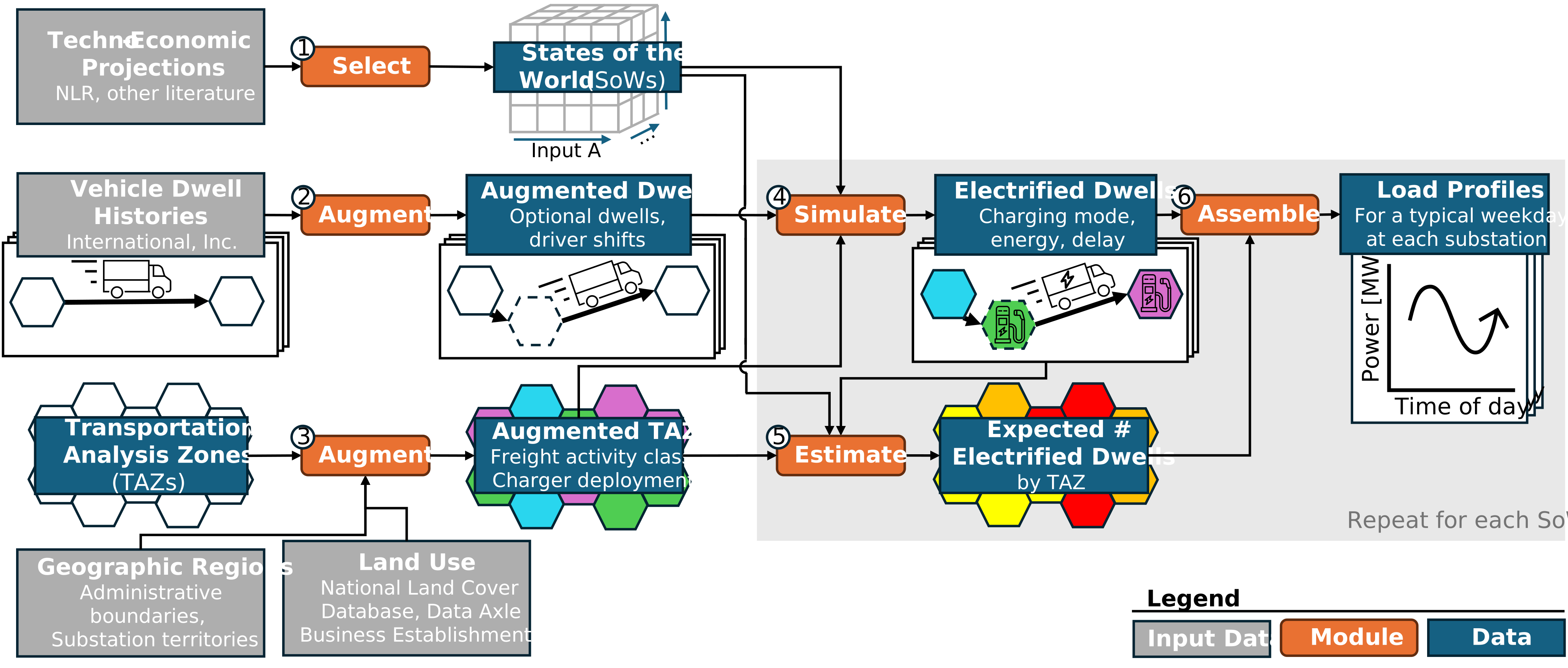
Module 1 — Select States of the World (`prepare_totals`, `build_scenarios`)

Selects a set of plausible states of the world (SoWs) to evaluate, generating 1024 quasi-random combinations using Sobol’ sequences (via OpenTURNS). Adoption rates by vehicle primary operating distance class are drawn from Beta distributions fit to NLR scenarios via a Gaussian copula. Other parameters (energy consumption rate, charger power at truck stops / depots / destinations, battery reserve) are sampled uniformly.

Module 2 — Augment Dwell Data (`describe_dwells`, `compute_routes`)

Augments vehicle dwell history data with optional dwells and with marked driver shifts. Coalesces spurious short dwells, marks driver shifts (≥6.9 hr breaks per FMCSA rules), and inserts optional dwells at truck stops along shortest-path routes computed by GraphHopper. Optional dwells are inserted between existing dwells separated by >50 miles, if a truck stop falls within 1 mile of the shortest path. This grew our dwell count by ~35%.

Module 3 — Augment TAZs (`describe_locations`)

Splits the continental U.S. into transportation analysis zones (TAZs) — H3 resolution-8 hexagons (~1/4-mile diameter) — and augments each with a freight activity classification and charger deployment. Classifies each TAZ into one of 22 freight activity classes:

Undeveloped / No establishments / No freight-intensive establishments / Truck stops
18 K-Means clusters of freight-intensive TAZs (based on NAICS employee counts)

Deploys chargers by freight activity class: truck-stop charging at truck-stop TAZs, destination charging at freight-intensive TAZs, depot charging per-vehicle based on a 30-day rolling dwell-time threshold.

Module 4 — Simulate Electrified Dwells (`electrify_trips`)

Simulates the e-HDT charging choices each vehicle in our dataset might have made, using a utility-maximization algorithm (inspired by Liu et al. 2022). The algorithm selects charging mode and energy amount at each dwell, trading off SoC maintenance against incurred delay, with look-ahead to the end of the current driver shift. Uses Numba JIT compilation for performance. Each SoW runs in ~25 minutes on a 4-core/64 GB machine.

Module 5 — Estimate Expected Electrified Dwells (`evaluate_impacts`)

Estimates the total number of electrified dwells expected in each TAZ, using the freight activity class. Fuses SoW adoption rates (from Module 1) with freight-activity-class-specific vehicle visit statistics from the observed data. Uses logistic regression with a numeric correction term to ensure consistency with known fleet-level adoption rates.

Module 6 — Assemble Load Profiles (`evaluate_impacts`)

Assembles charging load profiles for each substation from the simulated e-HDT vehicle histories by aggregating load profiles from the TAZs within each substation’s territory. Bootstrap-samples electrified dwells (100 draws, 95th percentile) to assemble 30-minute load profiles for each TAZ, then aggregates across all TAZs within each substation territory. Uses inverse propensity score weighting to correct for sampling bias in the telematics dataset. The final outputs are a set of charging load profiles for a typical weekday, one for each substation–SoW pair.

Input Data 

The model requires several external datasets, placed under data/01_raw/. The data catalog (conf/base/catalog.yml) defines where each dataset is expected.

Proprietary datasets (require a data-access agreement):

Dataset	Source	Pipeline(s)
International, Inc. telematics	Proprietary (contact International, Inc.)	`describe_dwells`, `describe_vehicles`, `compute_routes`, `electrify_trips`
Data Axle business establishments	Proprietary (contact Data Axle, Inc.)	`describe_locations`

Public datasets (freely downloadable):

Dataset	Source	Pipeline(s)
VIUS (Vehicle Inventory and Use Survey)	BTS	`prepare_totals`
NLR Ledna adoption scenarios	iScience 27 (2024) 109385	`prepare_totals`
HIFLD Electrical Substations	gem.anl.gov	`evaluate_impacts`
PG&E ICA maps	grip.pge.com	`evaluate_impacts` (PG&E territory only)
NLCD 2023 (National Land Cover Database)	USGS	`describe_locations`
Jason’s Law truck parking	BTS geodata	`describe_locations`, `compute_routes`
OpenStreetMap (North America)	Geofabrik	`compute_routes`, `describe_locations`

Note

Note on telematics data: The International, Inc. dataset is proprietary and cannot be redistributed. Researchers wishing to replicate this work should contact International, Inc. to request access, or adapt the pipeline to use a comparable telematics dataset with the same schema (vehicle ID, dwell TAZ, dwell start/end times, trip distance).

Note

Note on business establishments data: The Data Axle, Inc. dataset is proprietary and cannot be redistributed. Researchers wishing to replicate this work should contact Data Axle, Inc. to request access, or adapt the pipeline to use a comparable business establishment dataset with the same schema. The pipeline expects three tables joined on a shared establishment ID: a core table (ESTAB_ID, COMPANY, PRIMARY_NAICS_CODE, EMPLOYEE_SIZE__5____LOCATION, BUSINESS_STATUS_CODE, STATE), a geo table (ESTAB_ID, LATITUDE, LONGITUDE), and a relationships table (ESTAB_ID, PARENT_NUMBER).

Repository Structure 

LAUREL/
├── conf/                      # Kedro configuration
│   ├── base/                  # Shared parameters and data catalog
│   │   ├── catalog.yml        # ~860 dataset definitions
│   │   └── parameters_*.yml   # One parameter file per pipeline
│   ├── build_scenarios/       # Hand-written build specs (input to build_scenarios pipeline)
│   ├── scenarios/             # Per-task parameter overrides (mostly gitignored; validate/ included as example)
│   │   └── validate/          # Hand-built scenario example (not generated by build_scenarios)
├── data/                      # Data layers (Kedro convention; not committed)
│   ├── 01_raw/                # External source datasets
│   ├── 02_intermediate/       # Processed/formatted datasets
│   ├── 07_model_output/       # Per-scenario charging results
│   └── 08_reporting/          # Final visualizations and summaries
├── docs/                      # Sphinx documentation source
├── notebooks/                 # Exploratory Jupyter notebooks
├── scripts/
│   ├── setup/                 # Setup scripts for preparing model data before running scenarios
│   │   ├── submit_all.sh      # Submit steps 01-08 as a chain of dependent SLURM jobs
│   │   ├── 01_download_osm.sh
│   │   ├── 02a–08_*.sh        # Pipeline setup steps in execution order
│   │   └── ...
│   └── scenarios/             # Run scripts for scenario execution (e.g. validate.sh)
│       └── validate.sh        # Example: run script for the validate scenario
├── src/
│   ├── laurel/                # Main Python package
│   │   ├── datasets/          # Custom Kedro dataset classes (geospatial formats)
│   │   ├── models/            # Core algorithms (charging, dwell sets, sampling)
│   │   ├── pipelines/         # Nine Kedro pipelines (one per model module)
│   │   ├── routing/           # GraphHopper routing client and server management
│   │   ├── scenario_builders/ # Concrete ScenarioBuilder subclasses (one per scenario family)
│   │   ├── scenario_framework/# Abstract base classes, shell-script generator, I/O helpers
│   │   └── utils/             # Shared utilities (geo, H3, NAICS, time, ...)
├── tests/                     # pytest test suite
├── pyproject.toml             # Project metadata and dependencies
└── uv.lock                    # Locked dependency versions

Prerequisites 

Requirement	Notes
Python ≥ 3.12	Tested on 3.12
uv	Preferred package manager
Docker	Required only for the `compute_routes` pipeline (GraphHopper routing engine)
~200 GB disk space	For raw inputs + intermediate outputs for all 1024 SoWs
64 GB RAM	Minimum for running a single SoW through `electrify_trips` / `evaluate_impacts`
128 GB RAM	Recommended for `compute_routes`

For large-scale runs across all 1024 SoWs, an HPC cluster is strongly recommended (see HPC Execution (Sherlock)).

Installation 

# Clone the repository
git clone <repo-url>
cd LAUREL

# Install dependencies with uv (creates .venv automatically)
uv sync

# Or with pip into an existing environment
uv pip install -e .

To verify the installation:

uv run kedro info
uv run kedro pipeline list

You should see the eight pipelines: describe_vehicles, describe_dwells, compute_routes, describe_locations, prepare_totals, electrify_trips, evaluate_impacts, build_scenarios.

GraphHopper routing engine 

The compute_routes pipeline uses GraphHopper via Docker. Before running:

# Pull the GraphHopper Docker image
docker pull graphhopper/graphhopper

# The pipeline manages container startup/shutdown automatically
uv run kedro run --pipeline=compute_routes

The OSM road network file is downloaded for you by the download_inputs pipeline (see scripts/setup/01_download_osm.sh). Its location is the osm_north_america entry in conf/base/catalog.yml, which also pins the Geofabrik snapshot date; the same file is read by describe_locations, so it is downloaded once and shared.

Running the Model 

One-time data preparation 

Before running any scenario, the model data must be prepared. Submit the whole preparation chain with a single command from the repository root:

./scripts/setup/submit_all.sh

Each step in scripts/setup/ is submitted as a SLURM job that depends on the previous one (--dependency=afterok), so if a step fails or is cancelled SLURM automatically cancels everything downstream. Job logs are written to logs/slurm/<job_name>_<job_id>.log.

The chain runs these steps in order:

Script	Purpose
`01_download_osm.sh`	Download the OpenStreetMap extract for North America (skipped if already present)
`02a_describe_locations.sh`	Run the `describe_locations` pipeline (TAZ classification)
`02b_import_graph.sh`	Import the OSM graph into GraphHopper
`02c_preprocess_trips.sh`	Preprocess raw telematics trips
`03_prepare_routing.sh`	Start the GraphHopper routing server
`04_compute_routes.sh`	Run the `compute_routes` pipeline
`05_optional_stops.sh`	Insert optional truck-stop dwells along routes
`06_describe_dwells.sh`	Run the `describe_dwells` pipeline
`07_describe_vehicles.sh`	Run the `describe_vehicles` pipeline
`08_prepare_totals.sh`	Run the `prepare_totals` pipeline (SoW generation)

If a step fails, fix the cause and resume the chain from that step rather than starting over:

# Resume from a later step (the name must match the table above exactly)
./scripts/setup/submit_all.sh --from=04_compute_routes.sh

# Print the sbatch commands without submitting anything
./scripts/setup/submit_all.sh --dry-run

# Get an email as each step ends or fails
./scripts/setup/submit_all.sh --mail-user=you@stanford.edu

# Add a notification when each step starts, too
./scripts/setup/submit_all.sh --mail-user=you@stanford.edu --mail-type=ALL

--mail-type accepts any value SLURM does (BEGIN, END, FAIL, ALL, TIME_LIMIT, …) and defaults to END,FAIL. The flags apply to every job in the chain, so a full run sends one email per step.

The comments at the top of each step script can be used directly by SLURM to set its resource allocations (see HPC Execution (Sherlock)). Individual steps can also be submitted on their own with sbatch scripts/setup/<step>.sh – run this from the repository root so the scripts’ relative --output=logs/slurm/... resolves correctly – or run them as bash scripts directly.

Running a specific scenario 

To run a specific scenario, make sure that its configurations are in conf/scenarios/.... These configurations can be built by hand, like the one in conf/scenarios/validate/, or they can be generated using custom code via the build_scenarios pipeline. For example, here is the command to build the configurations for the sense_manage scenario set:

uv run kedro run --pipeline=build_scenarios --params=scenario_builders/sense_manage

This writes SLURM batch scripts to scripts/ and per-task config files to conf/scenarios/. Each array index corresponds to one SoW.

Once the configurations have been generated, you can run the scenarios one at a time using the --env flag to kedro run. The task_ directory at the bottom level is essential to allow SLURM’s job arrays to find the correct scenarios.

# Per-SoW simulation (run once per scenario)
uv run kedro run --pipeline=electrify_trips --env=scenarios/test/task_0
uv run kedro run --pipeline=evaluate_impacts --env=scenarios/test/task_0

Scenario run scripts 

The scripts/scenarios/ directory contains shell scripts for running individual scenarios. validate.sh is included as a tracked example. SLURM array scripts generated by build_scenarios (e.g. sense_manage.sh) land in the scripts/ root and are gitignored.

Scenarios 

Scenario definitions live in conf/scenarios/. Each scenario directory contains YAML files that override base parameters.

Scenario	Description
`sense_manage`	Main paper scenario: 1024 SoWs, adoption from NLR Beta+copula
`validate`	Validation run matching Broga et al. (2025) assumptions; hand-built (not generated by `build_scenarios`) — tracked in `conf/scenarios/validate/` as an example
`test`	Fast smoke-test scenario

Configuration 

To learn more about how parameter files are handled, and how scenarios override the base parameters, please see the Kedro documentation.

Data catalog (`conf/base/catalog.yml`)

Defines all ~860 datasets with their file paths and formats. Uses standard Kedro layers:

01_raw — source data (never modified)
02_intermediate — cleaned/formatted data
07_model_output — per-scenario simulation outputs
08_reporting — final outputs and visualizations

Per-scenario outputs are stored under data/07_model_output/<scenario_name>/<partition>/, where each partition directory contains one subdirectory per task_id, as partitioned Parquet datasets.

Pipeline parameters 

Each pipeline has a corresponding parameter file in conf/base/:

File	Controls
`parameters_describe_dwells.yml`	Dwell coalescing thresholds, shift detection
`parameters_describe_vehicles.yml`	Vehicle classification, depot detection window
`parameters_compute_routes.yml`	GraphHopper server config, optional dwell radius
`parameters_describe_locations.yml`	K-Means cluster count, NLCD thresholds, NAICS codes
`parameters_prepare_totals.yml`	SoW count, Sobol’ seed, Beta distribution parameters
`parameters_electrify_trips.yml`	Charging algorithm weights, delay caps
`parameters_evaluate_impacts.yml`	Bootstrap count, percentile, electrifiability criteria
`parameters_build_scenarios.yml`	SLURM configuration for HPC job arrays

Output Data 

After running evaluate_impacts for all 1024 SoWs, the outputs are organized as:

data/07_model_output/sense_manage/
├── dwells_with_charging_partition/   # Per-vehicle charging decisions
│   └── <task_id>/
├── report_by_region_quantiles/       # 30-min load profiles by substation
│   └── <task_id>/
└── report_by_region_summaries/       # Summaries of profiles by substation
    └── <task_id>/

The final reporting outputs (maps, policy analysis, validation figures) are in data/08_reporting/.

Cross-SoW aggregation 

To compute the 80th/20th percentile (“duty-to-serve-robust” / “used-and-useful-robust”) peak loads across all SoWs, aggregate the report_by_region_summaries datasets across task IDs. Example notebooks for this analysis are in notebooks/.

HPC Execution (Sherlock)

The full 1024-SoW run was computed on the Sherlock cluster at Stanford University. Each SoW takes ~25 minutes on 4 cores / 48 GB RAM.

Submitting jobs 

sbatch scripts/sense_manage.sh

GraphHopper on Sherlock (Apptainer)

HPC environments like Sherlock do not support Docker; use Apptainer instead. Loading the GraphHopper container requires a few manual steps:

Pull the container in sandbox mode:

apptainer pull --sandbox docker://israelhikingmap/graphhopper:10.2

Edit the container’s runscript to add cd /graphhopper at the very beginning. This works around Apptainer’s lack of support for Docker’s WORKDIR directive.
Edit /graphhopper/graphhopper.sh (inside the container) to restrict the .jar file search to the /graphhopper directory. The relevant line is near the bottom of the file where the JAR environment variable is set.

Once patched, point conf/base/parameters_compute_routes.yml at the Apptainer sandbox path instead of a Docker image name.

The paths handed to the container — the OSM extract via GraphHopper’s --input and the graph cache via --graph-cache — are resolved from data_dir before the container is launched. Do not write environment variables such as $SCRATCH into them: the command is built as an argument list with no shell, so nothing would expand them.

Development 

See CONTRIBUTING.md for development setup, running tests, linting, documentation builds, docstring standards, and guidance on adapting the pipeline to your own data.

Citation 

If you use this model or code in your research, please cite:

@article{passow2026laurel,
  title   = {Identifying indicators to inform proactive substation upgrades
             for charging electric heavy-duty trucks},
  author  = {Passow, Fletcher H. and Rajagopal, Ram},
  journal = {Applied Energy},
  year    = {2026},
  note    = {Submitted March 2026}
}

Acknowledgments 

The authors thank International, Inc. (especially Srinivas Gowda and Tobias Glitterstam) for sharing vehicle behavior data. This work was supported by the Bits & Watts Initiative at the Stanford Precourt Institute for Energy.

Computational resources were provided by the Sherlock cluster at Stanford University.